



Malicious software, or malware, refers to any program specifically designed to damage or disrupt a computer system without the consent or knowledge of its owner. The term “malware” encompasses a wide range of harmful software, which can be broadly classified into two categories: file infectors and stand-alone malware. The broader category of malware includes worms, backdoors, Trojans, rootkits, spyware, adware, and so on. These may be further subdivided into subcategories based on the harm they do (Saeed, 2020; Tahir, 2018).
Ransomware and malware have been utilized in various cyberattacks globally, with the number of ransomware variants rising at an alarming rate. A Symantec Security analysis revealed that the number of ransomware variants increased by 46% in 2017 (Beaman et al., 2021; Wani and Revathi, 2020). Because of the encryption process, ransomware victims cannot access their data until the ransom is paid. Attempts to analyse and identify malware have been studied for a long time. Different static and dynamic analysis techniques have been presented for malware (Begovic et al., 2023; Ispahany et al., 2024). Ransomware has similarities with other forms of malware but has distinct differences. In order to encrypt victim files, ransomware often performs a considerable number of actions on such files in a short amount of time. Further, once ransomware has attacked a system and specific encrypted data, it is impossible to decode the files without the appropriate decryption keys (Begovic et al., 2023; Humayun et al., 2021). While several methods have been developed for detecting and classifying malware, they are not effective for blocking ransomware since they only look for tells that indicate whether or not a file is malicious. Many computers have been compromised by malicious software in the modern digital age (Aboaoja et al., 2022; Bensaoud et al., 2024).
Malicious Software, or malware is designed to be harmful. It is widely used to control computers and other smart devices, expropriate valuable information, penetrate networks, and disrupt vital systems, among other things. Some examples of malware include viruses, warms, Trojans, spyware, bots, rootkit and ransomware. Computer Economics reported that the financial cost incurred due to malware-infected systems increased from $3.3 billion in 1997 to $13.3 billion in 2006, indicating a rising trend (Aqeel et al., 2022; Kikelomo et al., 2023). It’s important to note now that the various degrees of cyber-attacks from each year merit redefining the Year of Mega Breaches. For example, in 2016, WannaCry Ransomware Attack crippled systems in 150 plus countries, costing a variety of businesses millions of dollars in damage (Zimba and Chishimba, 2019). In fact, Cybersecurity Ventures forewarned in 2016 that the cost attributed to malware attacks would reach $6 trillion globally in 2021, massively increasing from the estimated $3 billion in 2015 (Bhusal and Rastogi, 2025).
Malware is a catch-all term that describes malicious attacks to computer systems (Saeed, 2020). Malware has been a growing challenge for the IT security field. According to Kaspersky Labs, in the past year, assaults on business PCs has exceeded 58% while network attacks reached 29%. Although hundreds of millions of malwares are discovered every day, the vast majority are developed from already-identified families (Yang et al., 2021). Packing, metamorphosis, and virtual technologies are the most common forms of malware obfuscation. These methods have been frequently used to avoid being detected by antivirus programmers (Brezinski and Ferens, 2023).
Antivirus vendors have generally embraced signature- and anomaly-based malware detection techniques. The signature approach offers a high degree of precision but cannot detect brand-new malware programmers and requires constant human updates to its feature library (Souri and Hosseini, 2018). Anomaly detection can be used to identify new viruses; however, it often suffers from a high false positive rate. Malware analysis is generally classified into two categories—static and dynamic—based on whether the malware is executed during the analysis. Static analysis examines binary files without executing the code, allowing for profiling the code flow and identifying the author’s writing style. However, it is vulnerable to obfuscation techniques that can disguise malicious intent (Bensaoud et al., 2024; Burnap et al., 2018).
Dynamic analysis effectively captures a program’s behavioural characteristics, even when encrypted or transformed. However, it requires extensive monitoring and logging, making it less efficient than static analysis (Urooj et al., 2021). Additionally, malware with activation conditions may evade detection. Machine learning has become a vital tool in malware analysis due to its success in other fields like image processing and speech recognition (Azeem et al., 2024; Gorment et al., 2023). It typically involves three phases: extracting static and dynamic properties, training a predictive model, and identifying unknown software. While machine learning can classify malware families, attackers can quickly generate new variants, raising key challenges: How can these variants be efficiently categorized? And how can newly release malware be detected?
The majority of current malware research is dedicated to dynamic analysis in sandboxes. This method involves running malicious software or an untrusted application in a sandbox to prevent severe system damage. There are potential drawbacks to this method, such as the fact that ransomware could be able to identify the sandbox and hence refuse to run at all. There is also the possibility that the command line parameters used by particular ransomware or malware may be unknown to us while they are testing in a sandbox environment. This work uses Machine Learning methods and suggests an ML-based strategy for malware classification and detection (Bayer et al., 2006; Or-Meir et al., 2020).
The increasing prevalence of malware, particularly ransomware, poses a significant threat to cybersecurity, leading to financial losses, data breaches, and system disruptions. Traditional malware detection techniques often struggle to accurately differentiate between benign and malicious files, especially when dealing with imbalanced datasets and evolving attack patterns (Qureshi et al., 2024; Smmarwar et al., 2024). This study aims to develop an improved malware detection method by integrating machine learning techniques with feature selection and data balancing strategies. The objective is to enhance detection accuracy, minimize false positives, and evaluate the effectiveness of various machine learning models in identifying malicious code. By implementing statistical validation techniques such as the T-test, this research seeks to establish the superiority of the proposed approach over conventional methods, ultimately contributing to more robust and efficient malware detection systems.
2. Related works
Various research studies across the world have studied how machine learning can detect and identify malware. To understand current machine learning strategies for malware detection, various research articles have been considered in this research study. Research suggested employed decision tree in n-gram patterns and outperformed both Naïve Bayes and support vector models in performance (Mohammed, 2023). Study also demonstrated a way to separate harmful software from safe software through API operation analysis (Lim, 2016). Similarly, the researchers employed association rules for analyzing honeytokens that had known characteristics (Catal et al., 2021). In a Hidden Markov Model is used to identify whether a given source code file is a variant of another source code file. Additionally, Profile Hidden Markov models successfully used for sequence analysis in bioinformatics and are used for a similar reason (Annachhatre et al., 2015). Neural networks have been explored for their ability to detect polymorphic malware, while Self-Organizing Maps (SOMs) have been used to identify malicious patterns in Windows executable files. Researchers have also proposed practical solutions to streamline the time-consuming process of model training for malware and virus classification (Shah et al., 2013). Support Vector Machines (SVMs) have proven to be effective tools for virus categorization, particularly when combined with high-dimensional n-grams extracted through dynamic analysis (Singh et al., 2016). This approach follows a two-step process to reduce dimensionality, improving classification accuracy.
Another demonstrated an innovative method for malware classification. There is a more sophisticated use of HMMs than grouping using k-means distance. The unique feature comes from the efforts of the four HMM modelers. Using a wide range of compilers and hand-crafted assembly language created not one but two potential mal- ware shapeshifter makers. The seven models used were GCC, MinGW, TurboC, Clang, TASM, NGVCK, and MWOR. Upon completion of the prototypes, each kind of malware is associated with its unique collection of “Opcode sequences” that are used to “teach” the model. These sequences has been given a score in a 7-tuple based on HMM models’ analysis. Variants of malware closer to the norms of the pedagogical dataset should get higher marks in return. These seven tuples are then input into the k- means algorithm, which organizes the examples of harmful code into categories. Finally, experimental results validate the efficacy of their method. It is a powerful tool for the automated labelling of images. Faulty programming conventions for pictorial representation have been used widely in several computer-related settings in science (Annachhatre et al., 2015). In addition to their importance in the field, these techniques are used to identify potentially harmful programmes.
Binary information can be changed into bitmap images. Following that, the bitmap image was converted into an entropy image by calculating the entropy values. They used to work with the visualization of malware through similarity graph (Han et al., 2014). The surface area for this function including malicious software and their constituent parts for their analysis, In a nutshell, generalized search trees based on wavelets (GIST) partition an image into its component pieces (Nataraj et al., 2011). Reflecting on the methods proposed by two different studies achieved classification accuracies of approximately 0.97–0.98, and the entropy-based approach was found to be faster to compute (Han et al., 2014; Nataraj et al., 2011). At the same time, it is faster to compute the former than the latter.
Thus, the former is the more efficient choice. New studies show that Opcode N-grams may provide defining features of a malware and viruses effectively (Ding et al., 2014). It is worth noting that in 2016, n-grams were extracted using similar techniques. Bi-normal separation and scaling is used in feature extraction. In addition, they gained through information gathering and using the rule of 2 to eliminate irrelevant choices. Considering the information, a 2 test may not only detect malware but precision in multi- classification up to 0.972. Numerous methods using windows apps exist. An application programming interface is a proposed solution.
Findings of Tian et al. (2010) determine how things work by interacting with their application programming interfaces and functional computer program code. Using a tracing tool to collect and analyze data from all the trace reports of the malware. They then attacked each API string and separated string values for each parameter. One way they could do this was by compiling an Archive of all viral string data in a single location. Moreover, it is guaranteed that the length of each feature vector in the input file is constant to be included in the vector; a string must have a value of ’1’ in the relevant position, as zero-based string indices are not provided. Their experiments confirmed that the random forest (RF) classifier provides the highest quality results. Despite the decreased accuracy, their analysis is contradicted with their data, which was closer to the truth (Cerda and Varoquaux, 2022). The term “intrusion response” (IR) is used to classify malicious programmes. They used a dynamic analysis method to use a combination of system operations and API requests in rapid succession to produce distinguishing features that may be found at several levels. In contrast to older methods, they would record every significant factor with great care. They captured both API and system calls in the documents then, we use IR theory and a weighted TF-IDF analysis to get characterizations of malware subfamilies. The outcomes of their laboratory methodology have better results than comparable methods. Hybrid analysis, which combines static and dynamic analysis methods, is beginning to get some attention from the academic community.
The researchers came up with an innovative approach. Using static and dynamic techniques, create a diagram depicting how information and commands are sent around (Hayashi et al., 2008). A newly developed virus employed obfuscation, and subsequent observations and testing verified two defining features of the approach. The approach has a high detection rate and an excellent building (Jia et al., 2023). Windows API calls are gleaned from a static analysis as they re-read people’s minds or analyze the actions of an attacker. Their testing reveals that only a small percentage of APIs, such as OpenProcess, Close- Handle, CopyFileA, and similar functions, are always seen together in harmful programs (Ye et al., 2018). Study illustrate that sample executables commonly have a similar set of opcodes in a specific malware family (Chen and Ren, 2023). Also, few opcodes are more prevalent in the malevolent distinction between malicious and safe executables. When analyzing malware, it is not uncommon for the vector to grow to a significant size, which may have a detrimental effect on the modelling process.
There is a wide range of feature selection techniques de- scribed in the literature. Strategies such as document frequency, information gain, and max-relevance algorithm have been utilized in many malware-detecting systems (Masud et al., 2011; Ye et al., 2008). Study also accomplished feature reduction using auto-encoders, lowering the memory and employing several classification techniques to attain incredible accuracy. Using many auto-encoders in a stack to remove background noise. Each model may be modelled after feature extraction for use by the classification algorithm as a feature vector in producing a virus detection model (Wang et al., 2016). Another study employed naive Bayes, J48, decision tree, k-nearest neigh- bour, multi-level perceptron and support vector machine on high-accuracy features were recovered using a dynamic analysis ratio of 96.8 per cent with J48 (Mohammed, 2023). The study created feature vectors using the byte n-gram approach, selecting features based on their frequency in documents and the leverage ratio. They achieved maximum accuracy by choosing the top 300 5-gram phrases with a decision tree and an artificial neural network (He et al., 2024). Genstatic analysis (sequence of opcode frequency) and dynamic characteristics (system call, error, etc.) were used to generate a composite feature vector from a dataset consisting of 1,000 malicious and 1,000 benign programmes (Kumar et al., 2019).
3. Materials and Methods
3.1 Ethical approval statement
No ethical approval was required to conduct the study.
3.2 Pre-processing
The dataset helps find malware by analyzing portable executable files. Our research began by obtaining files from Mendeley data to study harmful and safe executables. The dataset contains 5210 records in total out of which 2488 samples are benign and rest (2722) of the samples are malware with class 0 denoting representing benign and class 1 representing malware as shown in Table 1. The investigation process is shown in the figure 1.
Table 1. Number of benign and malware.
| Benign | Malware | Total |
| 2488 | 2722 | 5210 |
Careful dataset preparation is critical to improving the performance of learning models. We started by thorough examination of the dataset to verify any missing values or gaps data files. To maintain the integrity of data, incomplete or inconsistent data records were either omitted altogether or addressed through imputation. We normalize the dataset to let all feature values reach one common dimensional range. We employed Standard Scaler method to normalize feature values by subtracting the mean value from each part and dividing by the feature’s unit variations. Unit variance can be calculated simply by dividing all the data by the standard deviation. Standard Scaler method is effective with data that has Gaussian distribution, its calculations could change due to the outliers in the sample data. Standardization applies no adjustment to the initial dataset at present. The tool automatically transforms each feature to have a zero mean and adjusts the scale to one for each set. Devices that measure data at multiple scales can introduce bias and complicating model learning. To address this issue in model training we employed standard normalization on individual features.
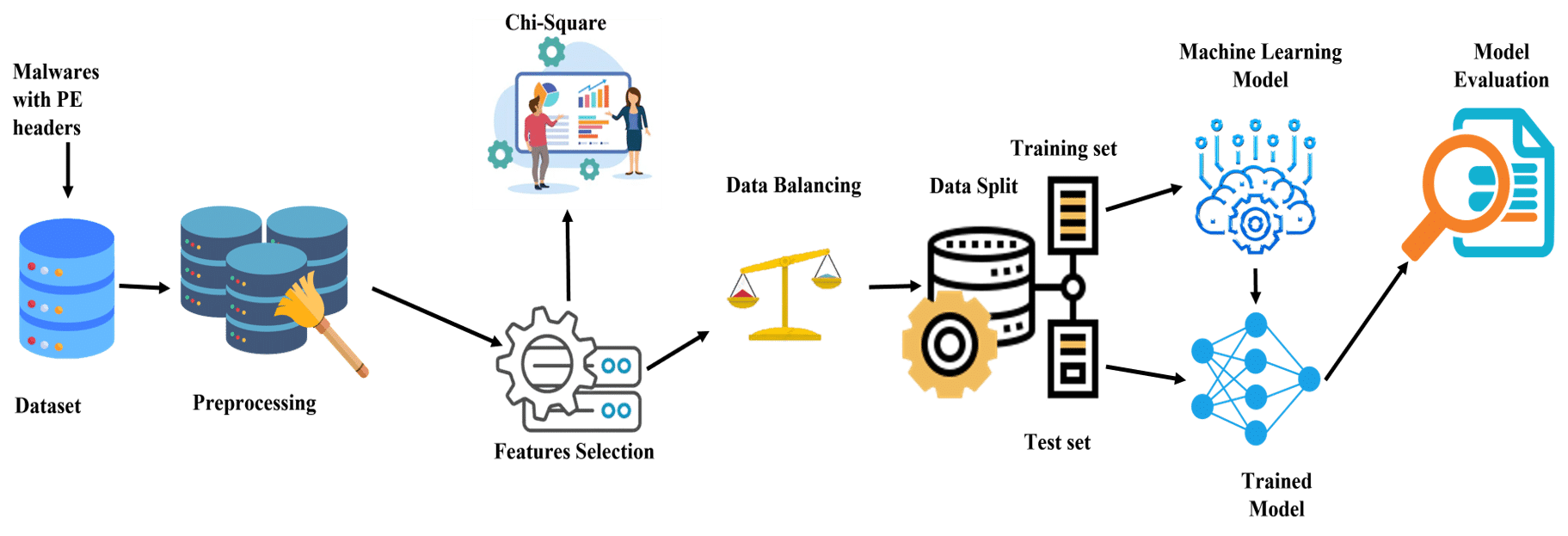
Figure 1. Architecture of the proposed approach.
3.3 Feature selection and data balancing
Due to the large number of possible features, feature selection is required in order to reduce the complexity of the training data. Chi2 feature selection procedures are used to determine the characteristics that are of the utmost importance. Chi2 is useful for categorical data because it assesses the independence of each feature with respect to the target variable. While Chi2 aims to analyze the original features directly, Principal Component Analysis (PCA) aims to reform the original features into a new set of orthogonal components. Comparing the results of the model becomes less complex when considering the importance of specific features on malware classification. In addition, the simplicity and computational efficiency of the Chi2 method make it the most convenient, especially when working with a large set of categorical features.
Table 2 displays the number of attributes that have a good match with Chi2’s selection of 15 malware characteristics. The number of characteristics that may be evaluated is established by looking at data from the real world. The objective of the feature selection process is to identify those aspects of the model that are determined by the response in the greatest degree. When two features are independent, the observed count will be relatively near to the projected count; hence, the Chi-square value will be lower in this scenario. So, the presence of a high Chi-Square score suggests that the assumption of independence is not valid. Conversely, a feature that has a higher Chi-Square value is more response-dependent, which makes it a more desirable candidate for model training.
Table 2. Number of features after Chi2.
| Features | Original | After Chi 2 |
| Total | 45 | 15 |
There is also an observation of class imbalance in our dataset, where benign samples are represented with 0 and malware samples as 1. This imbalance causes skewed results. Table 2 shows the number of class attributes in the dataset.
There are two ways to create a balanced dataset from an imbalanced one: one is to use under-sampling technique, and the other is to use over-sampling technique. Under-sampling technique creates statistical balance by reducing the number of samples in the majority class. When a dataset is large enough this technique is used. When modeling data, we can build an equalized dataset by keeping all the samples from rare classes and randomly picking samples from the majority classes. When we have limited data at hand then we can choose the oversampling technique. Expanding the smaller samples creates a data distribution that matches the majority class. These techniques of repletion boot- strapping and SMOTE help create new random samples instead of deleting duplicated as done in conventional practice. When available data falls short, we apply an approach called oversampling to adjust the imbalanced number. Making the lesser samples more plentiful level sets the data values. When building a dataset researchers use methods like repletion bootstrapping and SMOTE to create unique samples without removing common data points.
With SMOTE, new synthetic examples are crafted for the rare class, existing samples are used for interpolation in order to create real data points instead of just replicating existing data points. This technique also helps mitigate overfitting while maintaining the original proportion of the minority class. On the other hand, bootstrapping is done by random selection with replacement from the rare class, which augments it but does not alter the sample proportions within the original class structure. These techniques were adopted instead of simple replication methods because they preserve the accuracy of the model by having a more representative training set, which is critical in malware and benign sample classification. The statistics of balance dataset after applying up-sampling technique on the dataset is presented in Table 3. The dataset goes through preprocessing procedure to enhance the overall performance of the learning model. In the context of the data, some examples of preprocessing include scaling the data and selecting which characteristics to utilize.
Table 3. Number of class attributes.
| Benign | Malware | Total |
| 5444 | 5444 | 10888 |
When we need to pick several suitable features from available option Chi2 feature selection becomes applicable. The 2000 gene traits that drive successful learning matches are provided in Table II for readers to examine. In each experiment the selection of features occurs randomly based on chance alone. The model uses training information to create a Chi2 metric for assigning feature ranking importance. The findings are shown in Table 1. The model needs accessible data to analyze and learn from it. So, preprocessing the data is the first step then comes training phase. The ratio of data used for training and testing is 80:20. With limited available data the learning models train on just 80% of the total records. The other 20% of the data is then used for testing after model training. Because the dataset holds substantial data it can serve as input to train multiple models. After model training, test dataset is used evaluate model’s accuracy along with precision, recall and F1 Scores. In this study, many different machine learning models, including Bernoulli NaiveBayes, Guassian NaiveBayes, logistic regression, and SVM, were used to predicting malware. The table below, which is labelled as “Table IV,” provides a synopsis of the machine learning models that were used in this inquiry.
4. Results and Discussion
Our classification experiments help us establish a benchmark with which we compare our corpus analysis output. Our test shows each classifier’s F1 score, precision, and recall measurements side by side on separate charts. You can see the F1-Score performance along with precision and recall results for all models given in separate charts (Lee et al., 2024).
In contrast to the traditional machine learning models, our recommended feature-selection method uses random forest model which demonstrates improved performance without the need of any overfitting techniques. The categorization of malware in Logistic Regression makes the best use of our recommended categories. When contrasted with other methods of assessment, our recommended feature set assigns consistent significance to each of these factors. When compared to other models, our approach that is based on methods performs much better overall (Alsharif and Alharby, 2025; Sun et al., 2024). We compared the recommended approach to other ML models in which feature selection and data balancing were not carried out, our approach outperformed them. The findings of this investigation of without proposed method are shown in table 4.
Table 4. Comparative performance metrics of machine learning models without feature selection and data balancing.
| Model | Accuracy | K-Fold mean accuracy | SD | ROC_AUC | Precision | Recall | F1 score |
| Bernoulli | 83.68 | 85.07 | 0.85 | 0.83 | 0.85 | 0.82 | 0.83 |
| Logistic regression | 78.69 | 79.58 | 0.35 | 0.78 | 0.73 | 0.92 | 0.81 |
| Gaussian | 58.34 | 58.58 | 0.54 | 0.59 | 0.97 | 0.19 | 0.33 |
| SVM | 57.86 | 60.91 | 2.98 | 0.59 | 0.94 | 0.19 | 0.32 |
Most models perform poorly since they did not absorb training information when exposed to all attributes regardless of non-included features. Most of these features did not help the model learning works better (Carracedo-Reboredo et al., 2021). The model did not increase its performance when trained on complete features because most were excluded during training (Table 5).
Table 5. ML Models and their description.
| Model | Description |
| Bernoulli NaiveBayes | Bernoulli Naive Bayes is a part of the family of Naive Bayes. Only binary values are accepted. We may verify whether or not a value is a word that exists in a text as the most basic example. |
| Guassian NaiveBayes | The Bayes theorem is foundation for the probabilistic machine learning technique known as Nave Bayes. It is the expansion of naive Bayes to Gaussian Nave Bayes |
| SVM | Support vector machines, a group of methods for supervised learning, may be used for classification, regression, and outlier detection. The following are some of the benefits of using a support vector machine: Useful in areas with a lot of depth. Even if the number of dimensions exceeds the number of samples, it is still helpful. |
| Logistic regression | It is common practice to use logistic regression to solve categorization difficulties. Predictive analysis is used with probability theory to develop this regression model. One or more variables work together to produce a result that is most often understood in binary information. One or more independent variables may be linked with an approximation probability of using sigmoid logistic regression |
Figure 2 presents a performance comparison in terms of accuracy for different machine learning models that have been implemented.
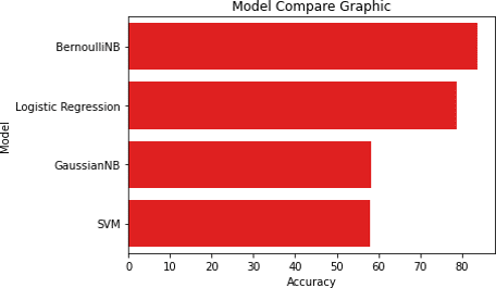
Figure 2. Accuracy comparison of various machine learning models without feature selection.
Figure 3 illustrates the trained model’s accuracy when applied to a dataset that consists just of the characteristics that were selected in the most efficient manner possible. In this particular instance, the model did not exhibit overfitting, and its findings may be seen for scrutiny. Figure 3 presents a comparison of the accuracy of all the well-trained models.
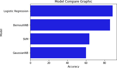
Figure 3. Accuracy comparison of various machine learning models with features selection.
When trained on data with just selected features, as shown in Table 6, most models had ROC AUC values that were close to 1, along with accuracy and recall that were almost equal to 1.
Table 6. Comparative performance metrics of machine learning models with feature selection and data balancing.
| Model | Accuracy | K-Fold mean accuracy | SD | ROC_AUC | Precision | Recall | F1 score |
| Logistic regression | 88.70 | 87.21 | 2.27 | 0.88 | 0.87 | 0.89 | 0.88 |
| Bernoulli NB | 85.85 | 88.47 | 0.39 | 0.85 | 0.86 | 0.85 | 0.85 |
| SVM | 63.72 | 62.31 | 0.19 | 0.63 | 1 | 0.26 | 0.42 |
| Gaussian NB | 60.05 | 59.44 | 0.84 | 0.59 | 0.96 | 0.20 | 0.33 |
Additionally, all the features were significantly linked with the class label and participated in the training process. Figure 4,5,6 show the results of ML models which have features selected on the basis of feature significance score determination. These graphs depict Recall, Precision and F1 score respectively.
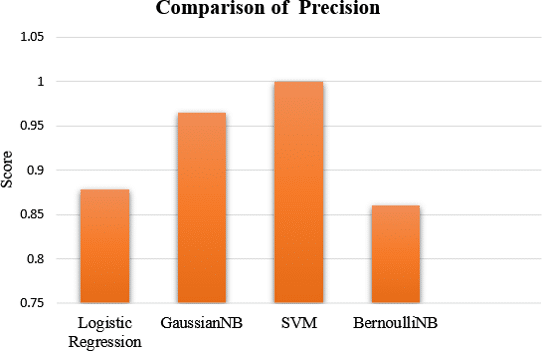
Figure 4. Precision comparison of various machine learning models.
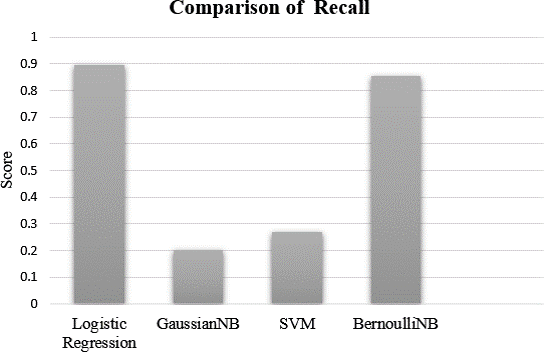
Figure 5. Recall comparison of various machine learning models.
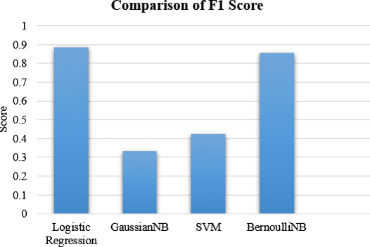
Figure 6. F1 score comparison of various machine learning models.
Whereas Figure 7 shows the combined results of performance in terms of F1 score, Precision, and Recall for different ML models. All the results from the ML models are received after applying K-fold cross validation.
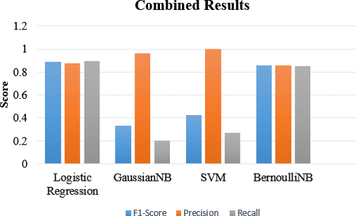
Figure 7. Combined evaluation of performance metrics of various machine learning models.
Even if our overall approach was good, SVM and Gaussian Naive Bayes did not perform well as anticipated. The unsatisfactory results on SVM performance might be due to its high dependence on the specified hyperparameters at the initial stages. In high-dimensional setting, the selection of the kernel as well as the regularization values is significant, for poor guessing usually leads to SVM having difficulties in capturing the non-linear features of the data (Guido et al., 2024; Nurjulaiha et al., 2025). Also, Gaussian Naive Bayes apply a normal distribution for the features, but a large number of features do not comply, resulting in underestimating the probabilities and hence the accuracy of misclassification. To overcome these shortcomings, further studies should be devoted to fine-tuning SVM hyperparameters, kernels, and regularization methods. For Gaussian NB, performance could also be improved by the transformation of features to fit the normal distribution more closely or other probabilistic models that are not restricted by rigid assumptions about distributions (Zhang, 2005). All these models can be included in the ensemble to take advantage of their shortcomings while compensating each other, which overall improves the validity of the detection.
4.1 Efficacy of proposed technique
The same dataset was utilized for validation, even though the importance of each feature has not been determined. T-tests were conducted to further validate the statistical significance of our findings. The results are shown in tables 5 and 6, along with an additional graph for further analysis. Figures 2 and 3 displays the comparison of the model that were carried out. A t-test, in which both the null hypothesis and an alternative hypothesis are examined, was performed to determine whether the recommended approach is statistically significant.
- Ho: Null hypothesis: The proposed technique will perform better.
- H1: Alternate hypothesis: The proposed technique will not perform better.
When ML models are used with feature selection using Chi2 and data balancing, the t-test accepted the null hypothesis. This indicates that the suggested method varies statistically from one in which just naïve ML techniques were used.
5. Conclusions
This study provides a method for the detection of malware that can classify between dangerous and safe data. The results of the testing show that our proposed method is successful in recognizing malicious code even when it is present in the same environment as files that seem to be completely benign, with a detection accuracy of up to 89%. Most of the recommended techniques are comprised of supervised learning, processed and balanced data, and data processing. To predict and classify cancer, the purpose of this research was to make use of an incomplete dataset. Based on the results of our studies, Logistic Regression performed better than any other machine learning methodology and did not result in an overfitting of the model when combined with the chi2 method as the primary feature extractor. There is a tendency for machine learning models to overfit when they are not informed of which attributes are most relevant. The findings that we obtained through verifying datasets and comparing the performance of our technique to those of well-known alternatives illustrate the method’s superiority and provide credibility to our statements.
Further studies must be done on the development of novel ensemble techniques. As defined, ensemble methods combined with the advantages of different classifiers to balance out the drawbacks of underlying models as well as to maximize the overall detection precision. At the same time, the use of deep learning (DL) frameworks like CNNs or RNNs is bound to improve feature extraction and classification accuracy, especially for sophisticated and high-dimensional data associated with modern malware.
Practically speaking, the most important next step is implementing the system in a real-world cybersecurity systems. Future work is required to ensure scalability and real time processing so that detection systems can function in systems with changing threat levels. Finally, the development of malware detection systems that automatically and opportunistically rethink their detection measures on the bases of newly available data is a prerequisite for effective defense against the new plethora of malware technologies.
